14.1 Polygon

14.1.1 Must not overlap

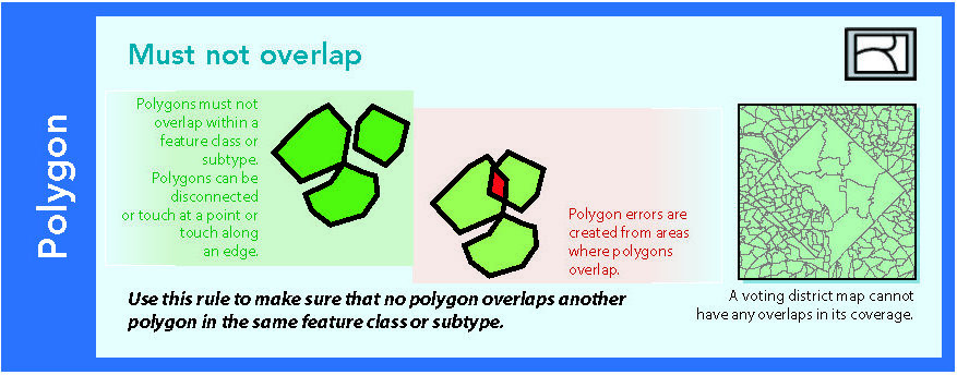
Figure 14.2: Source: Esri (2011)

In context of DE-9IM, this is a simple case. The polygon interiors should not overlap at all, everything else does not matter. Interior-Interior is the first of the 9 intersections, so the the intersection matrix as a code string would be: 2********. In the case of the example below:

set.seed(10)
nrows <- 10
circs <- data.frame(id = 1:nrows, x = rnorm(nrows), y = rnorm(nrows)) %>% st_as_sf(coords = c(2, 
    3)) %>% st_buffer(0.25)

circsplot <- ggplot(circs) + geom_sf(fill = "blue", alpha = 0.3) + geom_sf_text(aes(label = id)) + 
    theme_void()
circsplot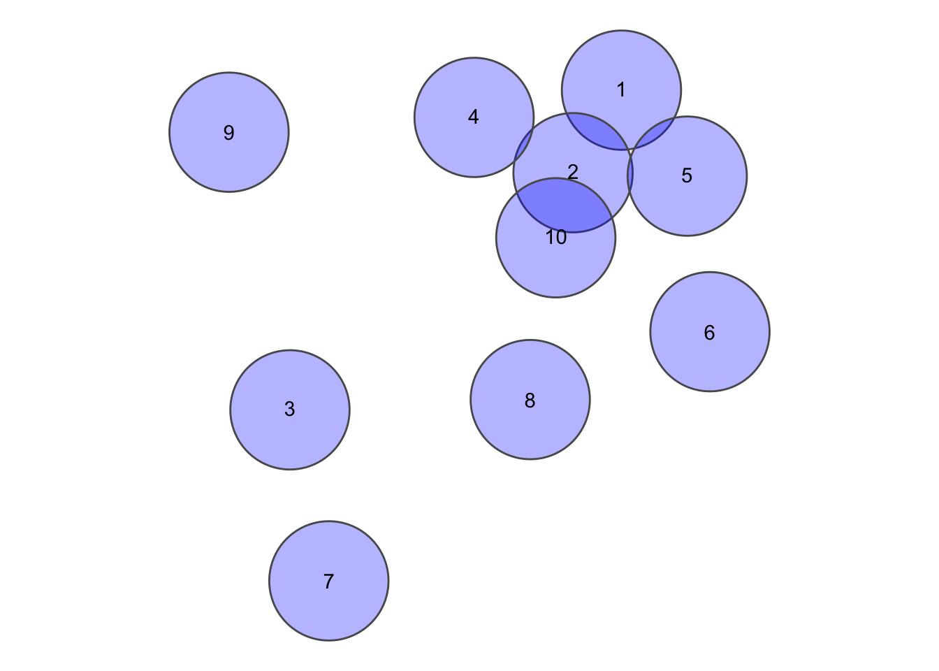

This gives us a sparse matrix as an output, which is esentially a list with the same length as the x, where each position is a vector of integers with the indicies of the features in y (which may equal to x) where the pattern matches.

st_relate(circs, pattern = "2********")

## Sparse geometry binary predicate list of length 10, where the predicate was `relate_pattern'
##  1: 1, 2, 5
##  2: 1, 2, 4, 5, 10
##  3: 3
##  4: 2, 4
##  5: 1, 2, 5
##  6: 6
##  7: 7
##  8: 8
##  9: 9
##  10: 2, 10

Setting sparse = FALSE returns a crossmatrix of all combinations.W

crossmatrix <- st_relate(circs, pattern = "2********", sparse = FALSE)
crossmatrix[1:6, 1:6]  # only showing 6 since this prints nicely

##       [,1]  [,2]  [,3]  [,4]  [,5]  [,6]
## [1,]  TRUE  TRUE FALSE FALSE  TRUE FALSE
## [2,]  TRUE  TRUE FALSE  TRUE  TRUE FALSE
## [3,] FALSE FALSE  TRUE FALSE FALSE FALSE
## [4,] FALSE  TRUE FALSE  TRUE FALSE FALSE
## [5,]  TRUE  TRUE FALSE FALSE  TRUE FALSE
## [6,] FALSE FALSE FALSE FALSE FALSE  TRUE

# Remove the diagonals since it's simply each feature tested against itself
diag(crossmatrix) <- FALSE
error <- which(crossmatrix, arr.ind = TRUE) %>% as.vector() %>% unique()


circsplot + geom_sf(data = circs[error, ], fill = "red", alpha = 0.3)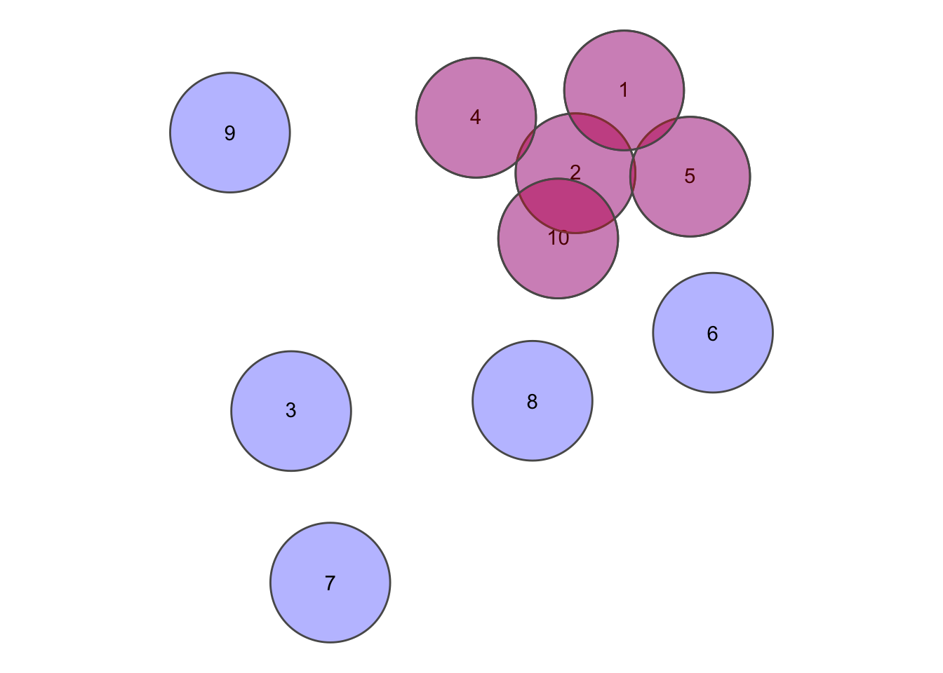

14.1.2 Must not have gaps

Figure 14.3: Source: Esri (2011)

Lets cosider the North Carolina Dataset for this question.

nc = st_read(system.file("shape/nc.shp", package = "sf"), quiet = TRUE)

ggplot(nc) + geom_sf() + theme_void()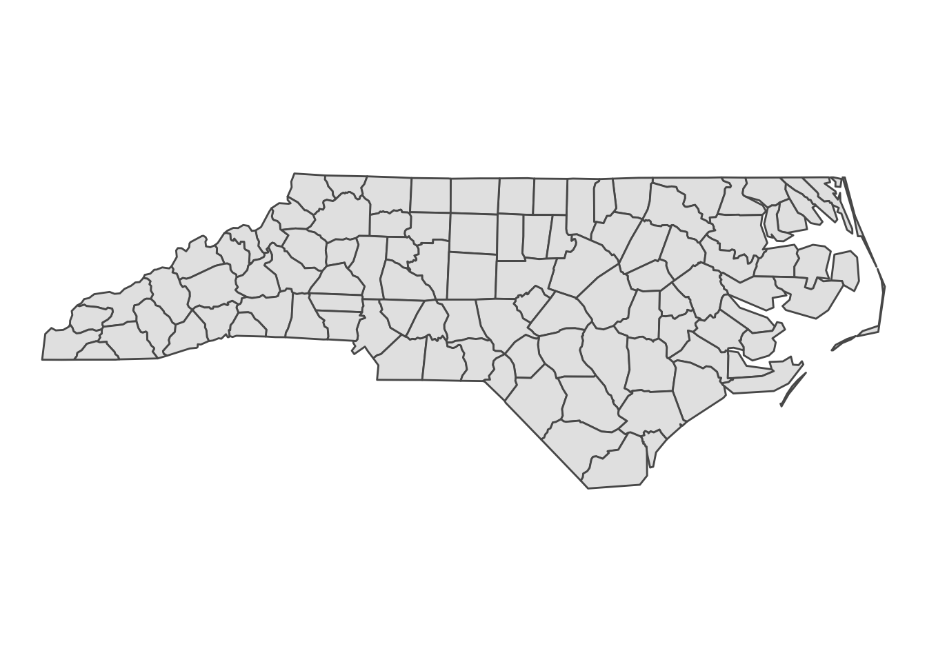

The first task is to dissolve all adjecent polygons together

nc_union <- st_union(nc)
nc_union

## Geometry set for 1 feature 
## geometry type:  MULTIPOLYGON
## dimension:      XY
## bbox:           xmin: -84.32385 ymin: 33.88199 xmax: -75.45698 ymax: 36.58965
## geographic CRS: NAD27

If the output is a multipolygon as it is the case here, it’s bad news, there are gaps. To check which parts are disconnected from each other, we can cast the multipolygon to a polygon (in ArcGIS Terms “Multipart to singlepart”), add a rowname for each part and colour it by rowname.

nc_singlepart <- nc_union %>% st_cast("POLYGON") %>% st_sf() %>% mutate(id = 1:n())

ggplot(nc_singlepart) + geom_sf(aes(fill = factor(id))) + labs(fill = "id") + theme_void()

But maybe we can live with these Islands in the state of North Carolina, since this is in fact an accurate representation of reality (the gaps are a result of the Atlantic Ocean). We must now check whether the individual geometries have holes. Here we can make use of the way polygons are defined in sf:

geometry with a positive area (two-dimensional); sequence of points form a closed, non-self intersecting ring; the first ring denotes the exterior ring, zero or more subsequent rings denote holes in this exterior ring

This means that the length of each Polygon geometry must be 1. A length of 2 or more would mean that there are one (or more) holes in the geometry. We can do this with any of the functions from the apply family, I prefer purrr:

map_lgl(nc_singlepart$geometry, ~length(.x) == 1)

## [1] TRUE TRUE TRUE TRUE TRUE TRUE

Let’s see what happens if we cut a hole into the polygons

holes <- nc_singlepart %>% st_union() %>% st_centroid() %>% st_buffer(0.5)

nc_holes <- st_difference(nc_singlepart, holes)

ggplot(nc_holes) + geom_sf() + theme_void()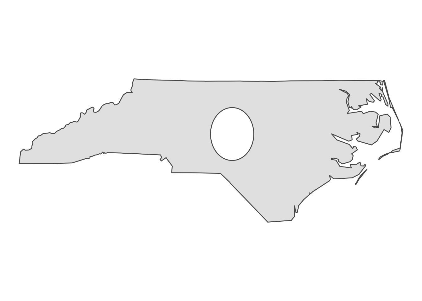

map_lgl(nc_holes$geometry, ~length(.x) == 1)

## [1] FALSE  TRUE  TRUE  TRUE  TRUE  TRUE

14.1.3 Contains point

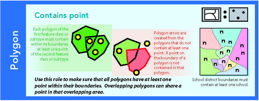
Figure 14.4: Source: Esri (2011)

14.1.4 Contains one Point

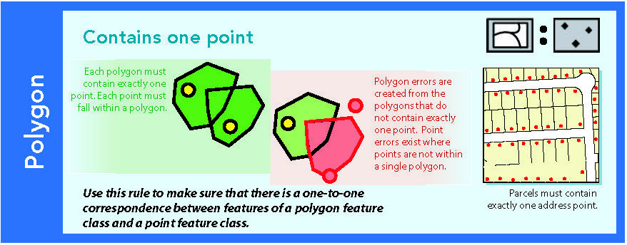
Figure 14.5: Source: Esri (2011)

14.1.5 Must be covered by feature class of

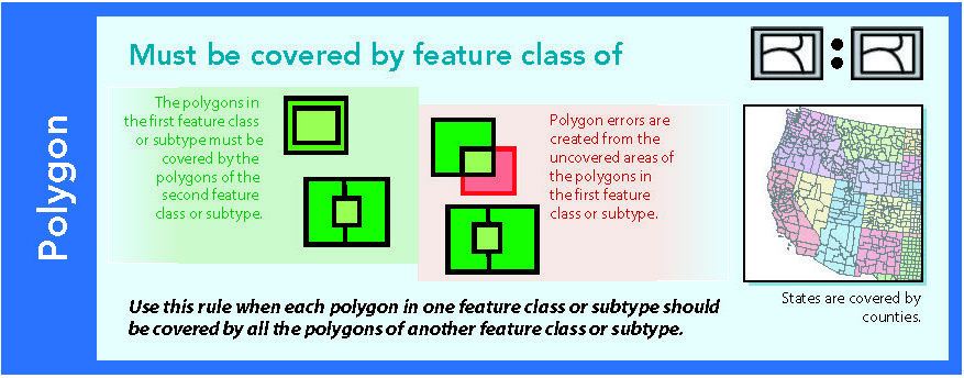
Figure 14.6: Source: Esri (2011)

14.1.6 Boundary must be covered by

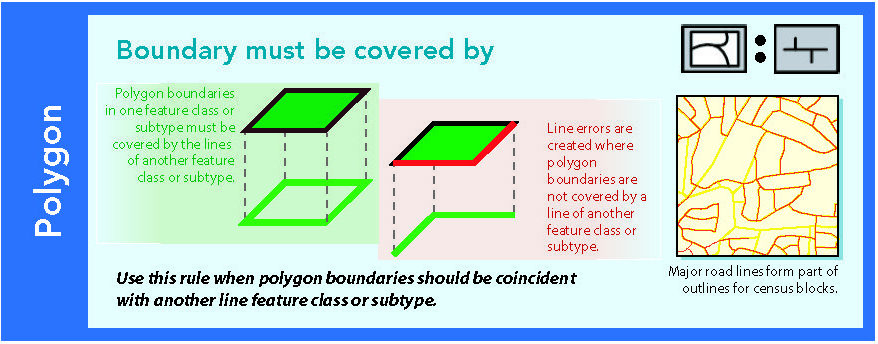
Figure 14.7: Source: Esri (2011)

14.1.7 Must not overlap with

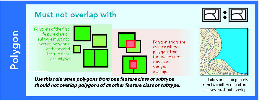
Figure 14.8: Source: Esri (2011)

14.1.8 Must be covered by

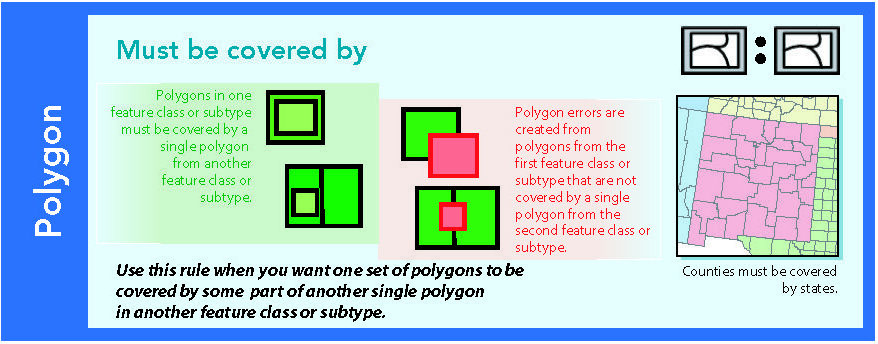
Figure 14.9: Source: Esri (2011)

14.1.9 Area boundary must be covered by boundary of

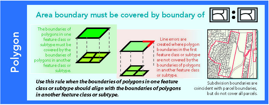
Figure 14.10: Source: Esri (2011)

14.1.10 Must cover each other

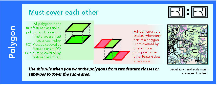
Figure 14.11: Source: Esri (2011)