9.1 Analysing Patterns Toolset

For this chapter, you will need the following R Packages:

library(arc2r)
library(sf)
library(ggplot2)

9.1.1 Spatial Autocorrelation (Global Morans I)

Here’s the function to calculate Morans I

morans_i <- function(sf_object, col) {
    require(sf)
    n <- nrow(sf_object)
    y <- unlist(st_set_geometry(sf_object, NULL)[, col], use.names = FALSE)
    ybar <- mean(y, na.rm = TRUE)
    dy <- y - ybar
    dy_sum <- sum(dy^2, na.rm = TRUE)
    vr <- n/dy_sum
    w <- st_touches(sf_object, sparse = FALSE)
    pm <- tcrossprod(dy)
    pmw <- pm * w
    spmw <- sum(pmw, na.rm = TRUE)
    smw <- sum(w, na.rm = TRUE)
    sw <- spmw/smw
    MI <- vr * sw
    MI
}

data("zweitwohnung_gemeinden")

zweitwohung <- st_set_crs(zweitwohnung_gemeinden, 2056)

zweit_plot <- ggplot(zweitwohung) + geom_sf(aes(fill = ja_in_percent), colour = NA) + 
    scale_fill_gradient2(low = "#2c7bb6", mid = "#ffffbf", high = "#d7191c", midpoint = 50, 
        breaks = c(0, 25, 50, 75, 100), limits = c(0, 100)) + labs(title = "Results from the 'Zweitwohungsinitiative'", 
    subtitle = "Percent in Approval", fill = "") + theme_void() + theme(legend.position = "bottom")

zweit_plot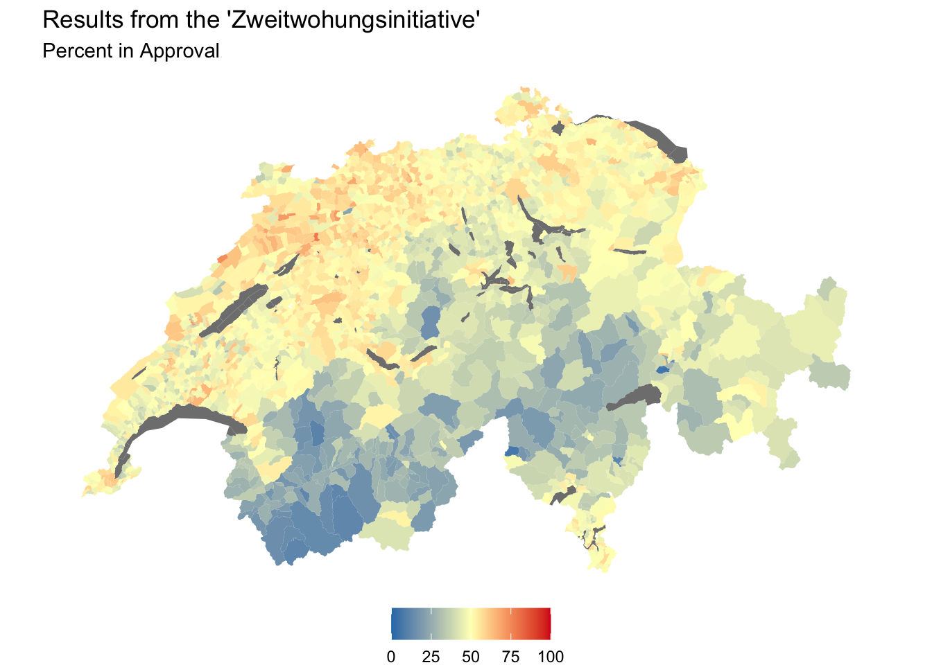

morans_i(zweitwohung, "ja_in_percent")

## [1] 0.6304227