13 DE-9IM

Thes named spatial predicates covered in chapter 12 are all based on the Dimensionally Extended 9-Intersection Model (DE-9IM).

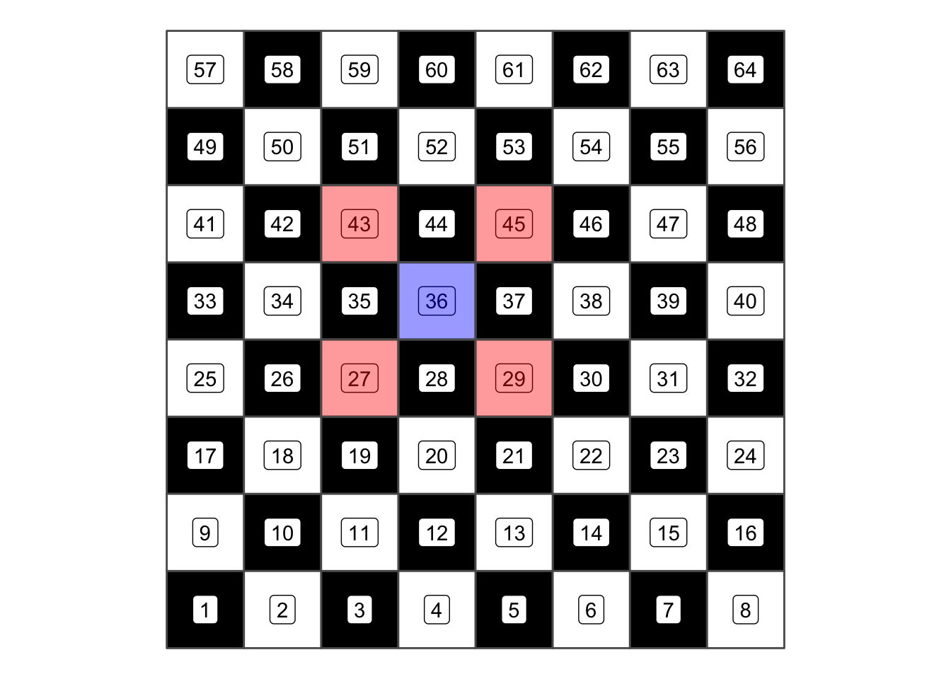
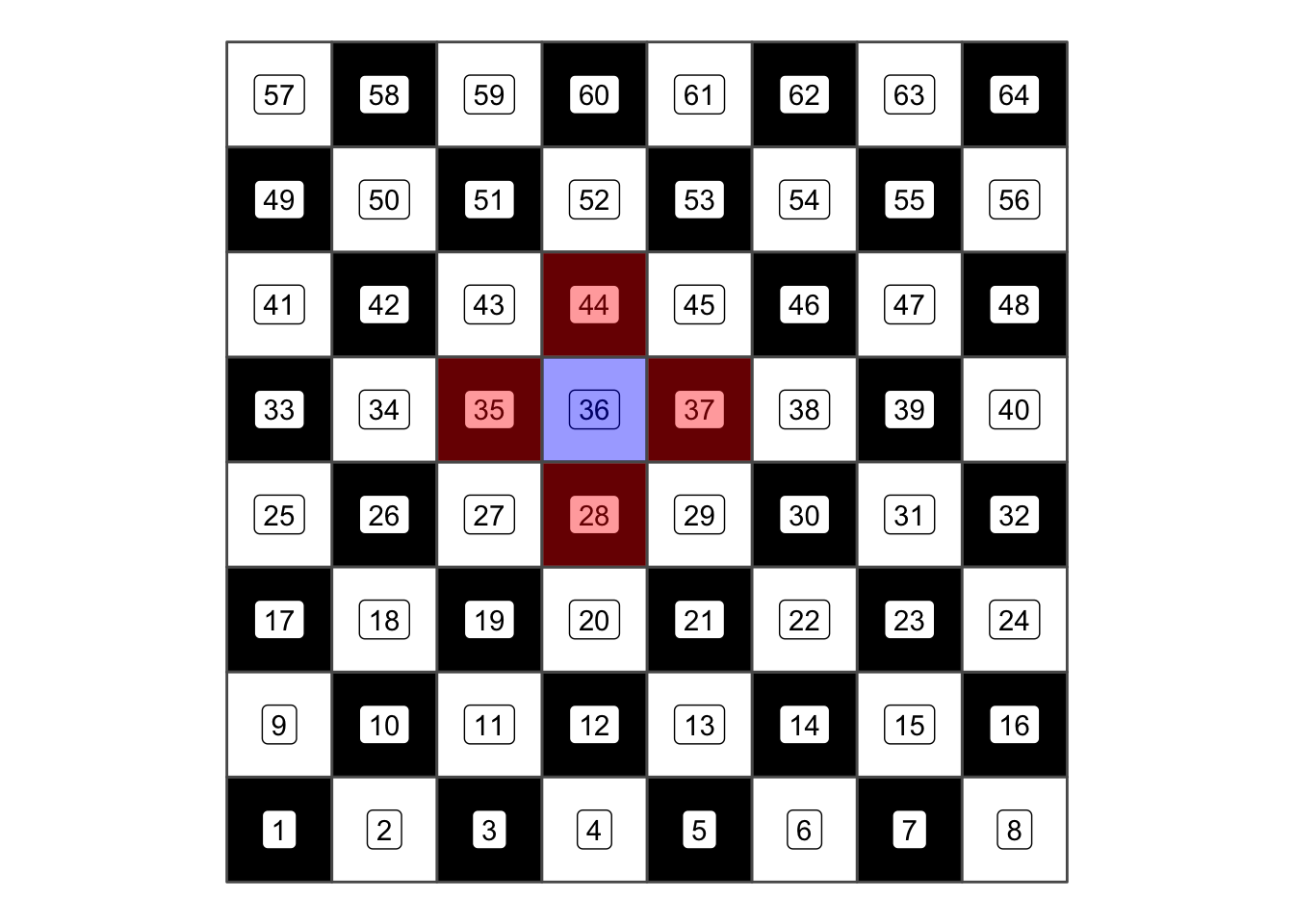
Regarding the chessboard example, we can imagine a chess piece placed on field #36. If this figure was a Queen or a King, all of the fields resulting from st_touches are reachable. In terms of contiguity, this is what is typically called the Queen’s or the King’s Case. However, this is might not the relationship that we are looking for: Say we would want to exclude the diagonal fields from our selection, the way a Rook would move in chess. How can we implement this in R?

None of the named topological relationships above (12) correctly describes this case (touches_but_not_at_edges or shares_boundary would be appropriate). In this case, we can use the Dimensionally Extended 9-Intersection Model (DE-9IM) to precisely formulate the relationship we are looking for: the Rooks Case.

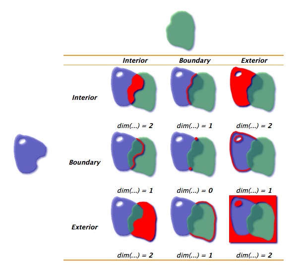
IN DE-9IM, the intersection of two objects is viewed at three levels for each object: The Interior, the Boundary and the Exterior (\(3^2= 9\), hence the name). These levels mean different things for Polygons, Lines or Points, but let’s just look at the simple case for now, polygons (which is the case for our chess fields). Take the example of two partially overlapping squares as shown below:

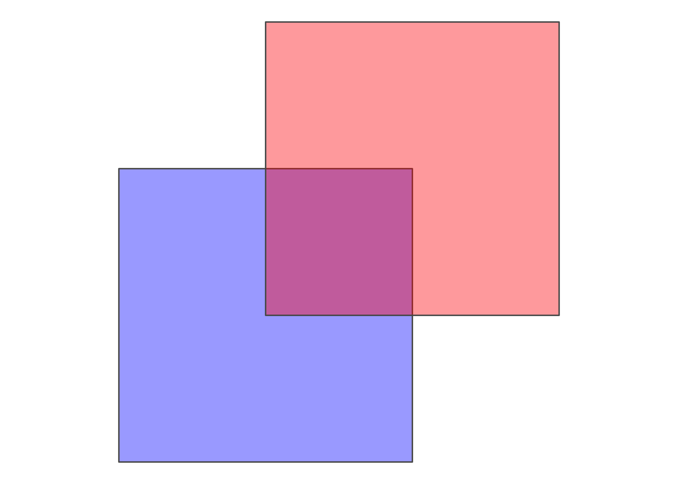
The interior of a polygon is the area inside the polygon. If the two areas overlap (as is the case of blue and red), the result from an intersection would also be a polygon. More formally: The dimesion of \(I(blue) \cap I(red)\) is an area. Areas get a value of 2, Lines 1 and points 0. If there is no intersection, the result equals to FALSE.

This was the first of 9 Intersections. Let’s look at the next one:

Interior of blue with the boundary of red:

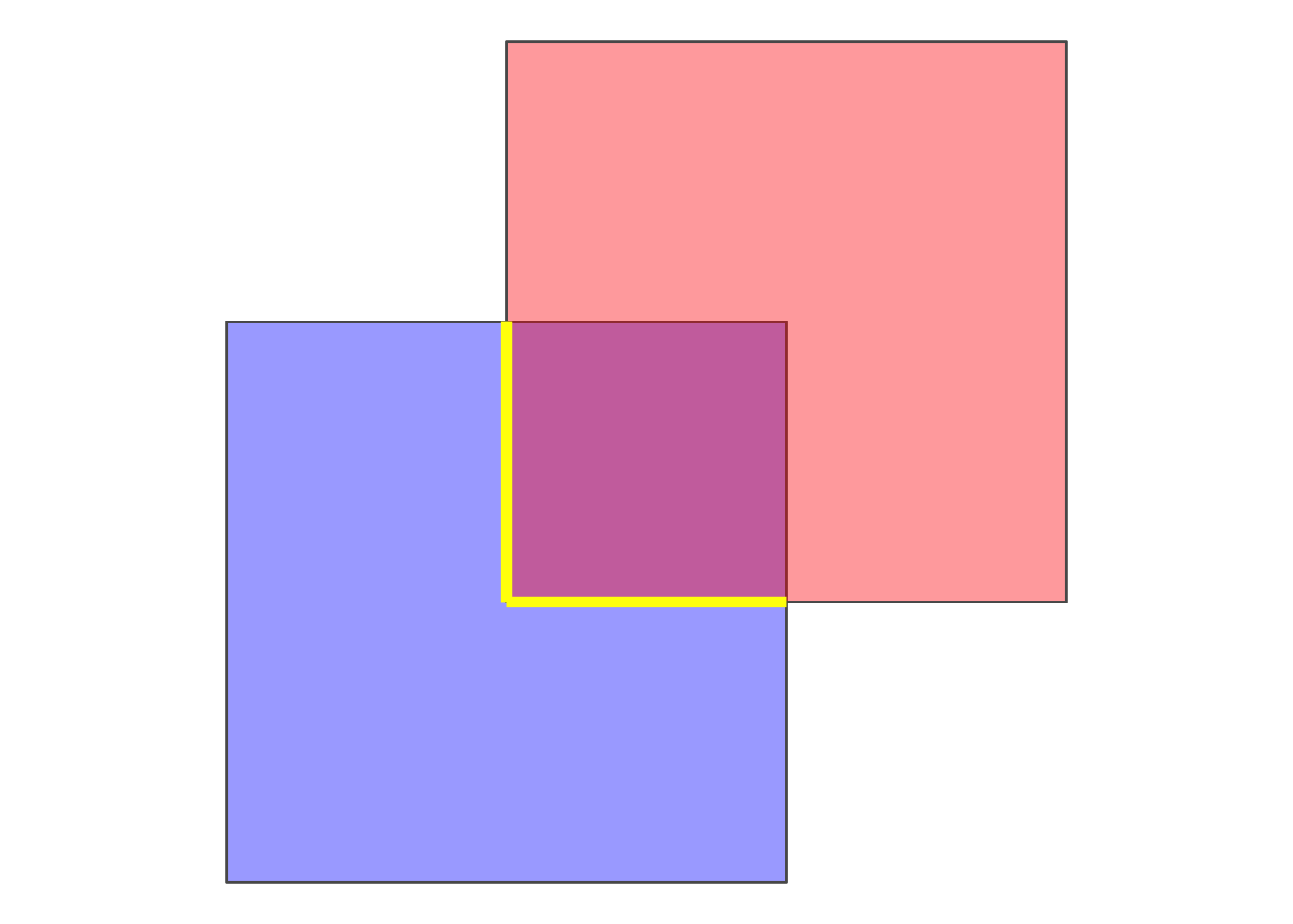
The resulting object has a dimenion “line,” i.e. 1. Formally: \(dim(I(blue) \cap B(red)) = 1\). Now just for the sake of looking at the third level (Exerior), let’s look at what this looks like:

p2_ls <- st_cast(p2, "LINESTRING")
p2_ls2 <- st_intersection(p1, p2_ls)

ggplot() + geom_sf(data = p1, fill = "blue", alpha = 0.4) + geom_sf(data = p2, fill = "red", 
    alpha = 0.4) + geom_sf(data = st_difference(p1, p2), fill = "yellow", lwd = 2) + 
    theme_void()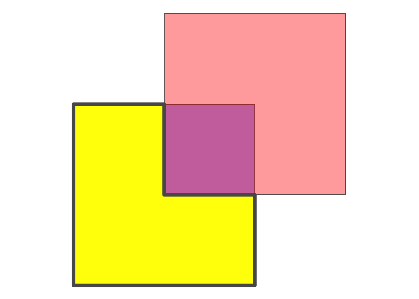

The resulting object is again an area, i.e. 2. Formally \(dim(I(blue) \cap E(red)) = 2\).

If we go through all intersections of Interior, boundry and Exterior of both geometries, we can denote for each comination what type of dimesion we “allow.” This can be either 0 (for points), 1 (for lines) or 3 (for areas) or TRUE (for either of these), or FALSE (for none of these) or * (for "I dont care).

13.0.0.1 Rooks Case

If we go throught the all nine combinations of the DE-9IM, this is what defines the rooks case:

	Interior	Boundary	Exterior
Interior	nothing	don’t care	don’t care
Boundary	don’t care	Line	don’t care
Exterior	don’t care	don’t care	don’t care

We can now write this into a string, starting from the top left: F***1****

Now that we have this string, we case use st_relate()and specify the string as the pattern we are looking for:

st_relate(chessboard[36, ], chessboard, pattern = "F***1****")

## Sparse geometry binary predicate list of length 1, where the predicate was `relate_pattern'
##  1: 28, 35, 37, 44

Which visually gives us this pattern:

Because this was so much fun, let’s also have a look at the opposite, the Bishops Case.

13.0.0.2 Bishops Case

	Interior	Boundary	Exterior
Interior	nothing	don’t care	don’t care
Boundary	don’t care	Point	don’t care
Exterior	don’t care	don’t care	don’t care

st_relate(chessboard[36, ], chessboard, pattern = "F***0****")

## Sparse geometry binary predicate list of length 1, where the predicate was `relate_pattern'
##  1: 27, 29, 43, 45

Visually: