6.2 Overlay Toolset

From the docs (Esri 2020):

The Overlay toolset contains tools to overlay multiple feature classes to combine, erase, modify, or update spatial features, resulting in a new feature class. New information is created when overlaying one set of features with another. All of the overlay operations involve joining two sets of features into a single set of features to identify spatial relationships between the input features.

For this chapter, you will need the following R Packages:

library(arc2r)
library(sf)
library(dplyr)
library(ggplot2)

6.2.1 Spatial Join

Esri (2020) describes Spatial Join as follows:

Joins attributes from one feature to another based on the spatial relationship. The target features and the joined attributes from the join features are written to the output feature class.

Say you have two datasets, haltestelle_bahn and kantonsgebiet as shown below.

data("haltestelle_bahn")
data("kantonsgebiet")


head(haltestelle_bahn)

## Simple feature collection with 6 features and 1 field
## geometry type:  POINT
## dimension:      XY
## bbox:           xmin: 2694932 ymin: 1263039 xmax: 2713408 ymax: 1289090
## projected CRS:  CH1903+ / LV95
##                name                geometry
## 1          Thayngen POINT (2694932 1289090)
## 2            Ramsen POINT (2703768 1285024)
## 3        Hemishofen POINT (2704726 1281756)
## 4 Weberei Matzingen POINT (2711701 1265116)
## 5         Matzingen POINT (2712529 1264372)
## 6         Jakobstal POINT (2713408 1263039)

head(kantonsgebiet)

## Simple feature collection with 6 features and 1 field
## geometry type:  POLYGON
## dimension:      XY
## bbox:           xmin: 2494306 ymin: 1075268 xmax: 2833858 ymax: 1268609
## projected CRS:  CH1903+ / LV95
##         NAME                       geometry
## 1 Graubünden POLYGON ((2735216 1194955, ...
## 2       Bern POLYGON ((2595242 1169313, ...
## 3     Valais POLYGON ((2601808 1136117, ...
## 4       Vaud POLYGON ((2555093 1138713, ...
## 5     Ticino POLYGON ((2727359 1119219, ...
## 6 St. Gallen POLYGON ((2716175 1240719, ...

plot(st_geometry(kantonsgebiet))
plot(haltestelle_bahn, add = TRUE, col = "blue", pch = 20)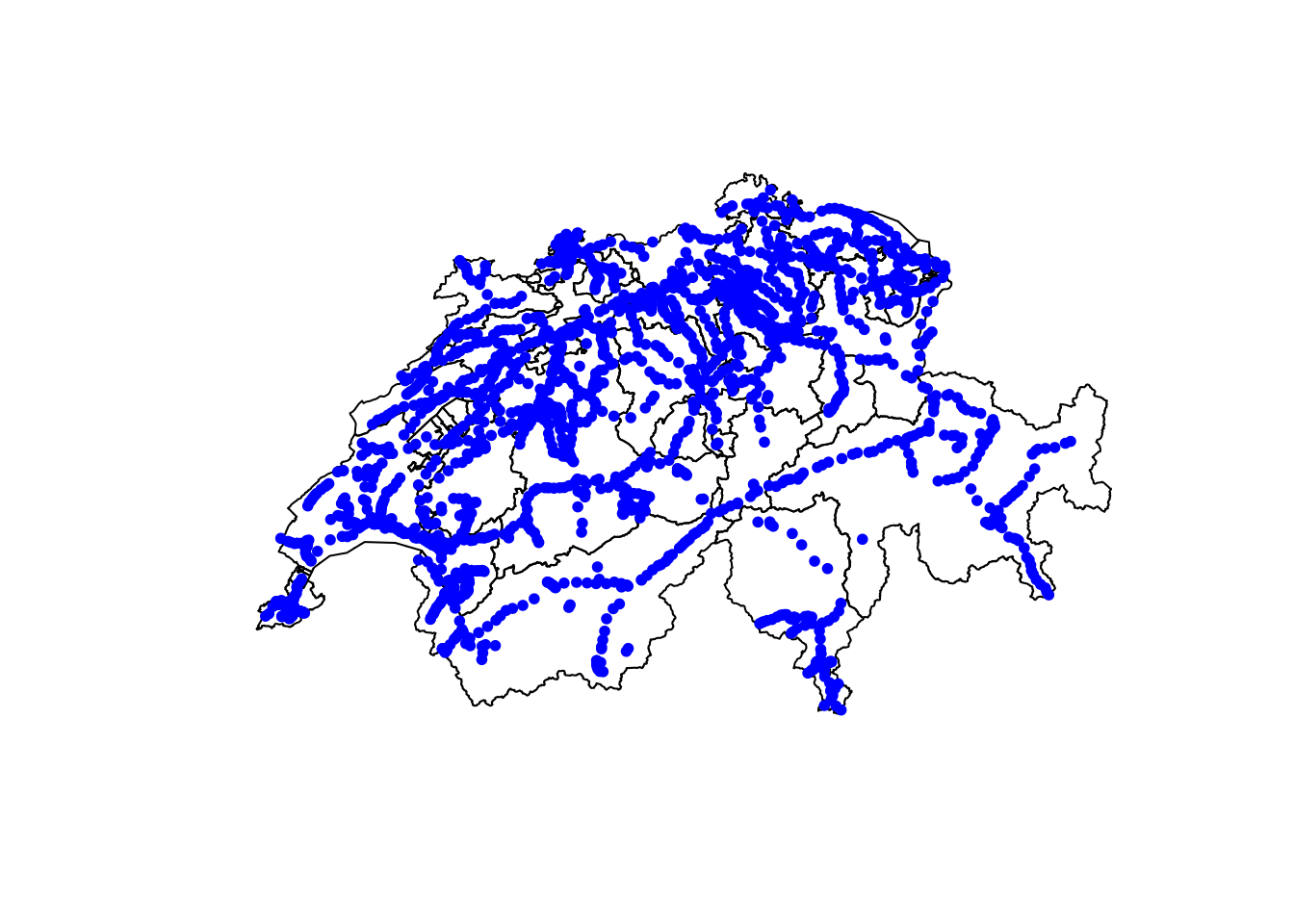

For each point in haltestelln_bahn, we would like to know the name of the canton in which it is located. In R, the function used to join two datastes is st_join(x,y). If you have to different data types (e.g. Points and Polygons) the first question you have to ask yourself is: what data type should the output be? The datatype of x determines what the output datatype is. So with the above data: Say for each point, we want to know the Name (name) of the “Canton” in which it lies. This means the output is a point dataset. We therefore write:

haltestelle_bahn_join <- st_join(haltestelle_bahn, kantonsgebiet)


haltestelle_bahn_join

## Simple feature collection with 3134 features and 2 fields
## geometry type:  POINT
## dimension:      XY
## bbox:           xmin: 2488908 ymin: 1076850 xmax: 2817389 ymax: 1289090
## projected CRS:  CH1903+ / LV95
## First 10 features:
##                     name         NAME                geometry
## 1               Thayngen Schaffhausen POINT (2694932 1289090)
## 2                 Ramsen Schaffhausen POINT (2703768 1285024)
## 3             Hemishofen Schaffhausen POINT (2704726 1281756)
## 4      Weberei Matzingen      Thurgau POINT (2711701 1265116)
## 5              Matzingen      Thurgau POINT (2712529 1264372)
## 6              Jakobstal      Thurgau POINT (2713408 1263039)
## 7            Wiesengrund      Thurgau POINT (2713771 1262367)
## 8                  Wängi      Thurgau POINT (2714128 1261715)
## 9               Rosental      Thurgau POINT (2715765 1261315)
## 10 Münchwilen Pflegeheim      Thurgau POINT (2717089 1260114)

The following visualisation shows that each point has inherited the Name of the according Canton.

ggplot() + geom_sf(data = kantonsgebiet) + geom_sf(data = haltestelle_bahn_join, 
    aes(colour = NAME))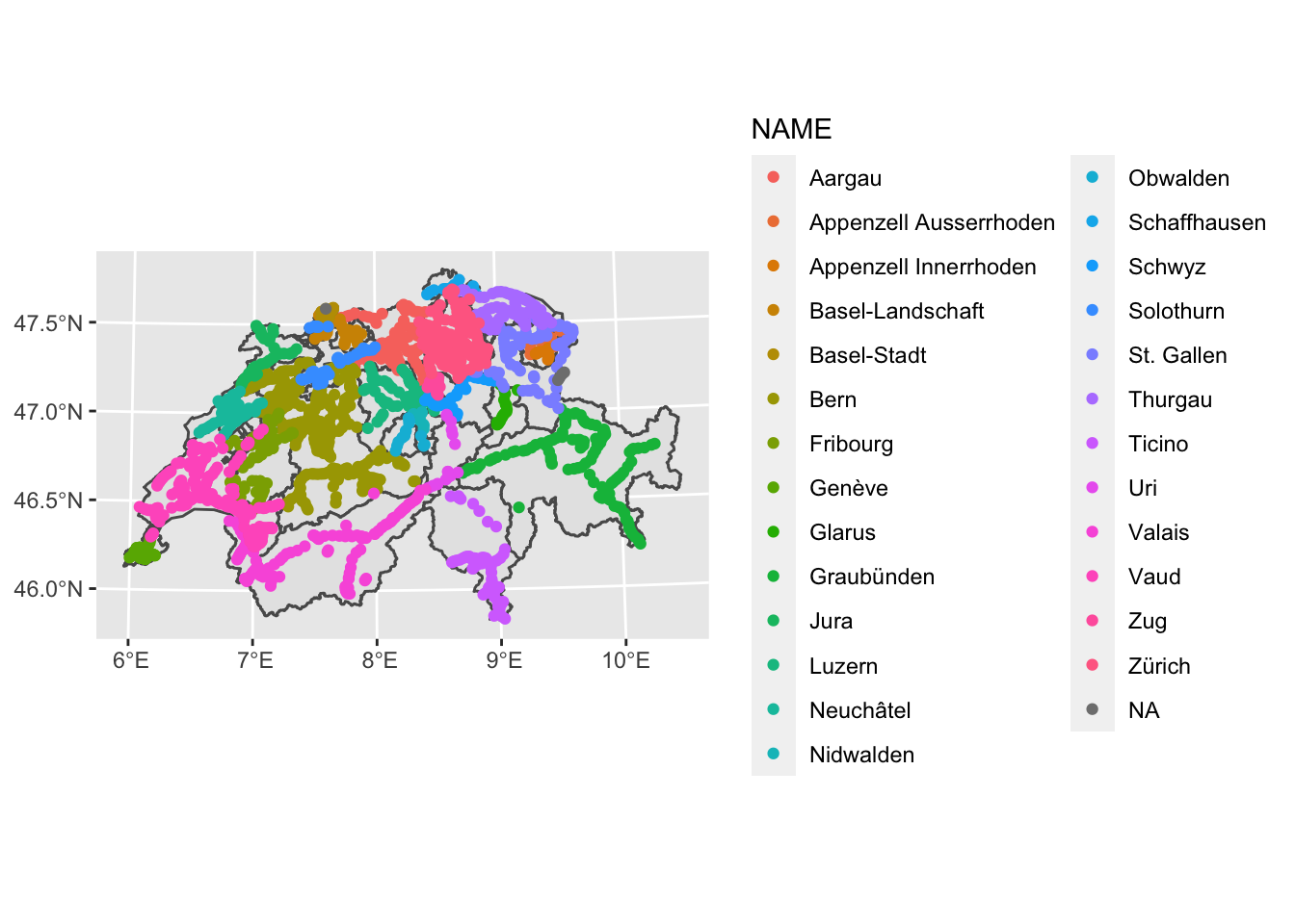

By default, the spatial relationship between haltestellen_bahn and kantonsgebiet was that of an “intersection” (this is also de default in ArcGIS). However, we can do spatial joins with other relationships as well: These relationships are commonly known as “spatial predicates.”

ArcGIS Term	R Spatial Predicate
Intersect	st_intersect
Intersect 3D	\(^1\)
Within a distance	st_is_within_distance
Within a distance geodesic	\(^2\)
Within a distance 3D	\(^1\)
Contains	st_contains
Completely contains	st_contains_properly
Contains clementini	\(^2\)
Within	st_within
Completely within	\(^2\)
Within clementini	\(^2\)
Are identical to	st_equals
boundry touches	st_touches
Share a line segment	\(^2\)
Have their center in	\(^2\)
Closest	st_nearest_feature
Closest geodesic	\(^2\)

\(^1\) All binary predicates only work on 2D Objects (see this issue)

\(^2\) We haven’t figured out which Spatial Predicate matches this ArcGIS term.