7.1 General Toolset
For this chapter, you will need the following R Packages:
library(arc2r)
library(sf)
library(ggplot2)
library(dplyr)
7.1.1 Sort
Sorting out features in ascending or descending order seems a quite primitive operation in any programming language or software package. Even though it is indeed primitive, it is also quite important for filtering and cleaning our datasets. In ArcGIS pro this operation is performed using the tool Sort, which is part of the General toolset of the Data Managenent Toolbox. Below we present how we can perform the aforementioned operation using R. For our example we use the Simple Feature object bezirke, which depicts the districts within the country of Switzerland. Furthermore for performing the sorting operation, we use the record(column) that represents the area (in square km) of every of the districts.
# Read the dataset depicting the districts (Bezirke) in the country of
# Switzerland
data("bezirke")

# sort the dataset based on the Area in ascending order
bezirke_asc <- bezirke[order(bezirke$area_km2), ]
head(bezirke_asc)
## Simple feature collection with 6 features and 4 fields
## geometry type: MULTIPOLYGON
## dimension: XYZ
## bbox: xmin: 2574333 ymin: 1210642 xmax: 2744654 ymax: 1279605
## z_range: zmin: -1.455192e-11 zmax: -1.455192e-11
## CRS: NA
## NAME OBJEKTART OBJECTID area_km2 geom
## 68 St. Gallen Bezirk 153 0.1150075 MULTIPOLYGON Z (((2744592 1...
## 133 Höfe Bezirk 1 0.1312150 MULTIPOLYGON Z (((2701415 1...
## 186 Schaffhausen Kanton 176 0.2405185 MULTIPOLYGON Z (((2707903 1...
## 104 Seeland Bezirk 9 0.4128530 MULTIPOLYGON Z (((2575776 1...
## 119 Wil Bezirk 145 0.5292165 MULTIPOLYGON Z (((2732986 1...
## 131 Höfe Bezirk 43 0.5612065 MULTIPOLYGON Z (((2702572 1...# sort the dataset based on the Area in descending order
bezirke_desc <- bezirke[order(-bezirke$area_km2), ]
head(bezirke_desc)## Simple feature collection with 6 features and 4 fields
## geometry type: MULTIPOLYGON
## dimension: XYZ
## bbox: xmin: 2580900 ymin: 1128447 xmax: 2833842 ymax: 1219106
## z_range: zmin: -1.455192e-11 zmax: -1.455192e-11
## CRS: NA
## NAME OBJEKTART OBJECTID area_km2
## 15 Surselva Bezirk 13 1373.7973
## 9 Interlaken-Oberhasli Bezirk 15 1231.6744
## 2 Engiadina Bassa/Val Müstair Bezirk 74 1197.5201
## 171 Uri Kanton 159 1076.0927
## 4 Maloja Bezirk 183 973.7269
## 52 Bern-Mittelland Bezirk 89 939.6023
## geom
## 15 MULTIPOLYGON Z (((2713720 1...
## 9 MULTIPOLYGON Z (((2629665 1...
## 2 MULTIPOLYGON Z (((2812980 1...
## 171 MULTIPOLYGON Z (((2684185 1...
## 4 MULTIPOLYGON Z (((2775675 1...
## 52 MULTIPOLYGON Z (((2587852 1...The beauty of R is that offers more than one option to perform a specific operation. In the example above, for performing the sorting operation, we used a simple subsetting method integrated within the so called base R. Nevertheless using the the function arrange() of the dpyr package we will be able to produce the exact same result.
# sort the dataset based on the Area in ascending order
bezirke_arrange_asc <- arrange(bezirke, area_km2)  # by default the function sorts in ascendind order
head(bezirke_arrange_asc)
## Simple feature collection with 6 features and 4 fields
## geometry type: MULTIPOLYGON
## dimension: XYZ
## bbox: xmin: 2574333 ymin: 1210642 xmax: 2744654 ymax: 1279605
## z_range: zmin: -1.455192e-11 zmax: -1.455192e-11
## CRS: NA
## NAME OBJEKTART OBJECTID area_km2 geom
## 1 St. Gallen Bezirk 153 0.1150075 MULTIPOLYGON Z (((2744592 1...
## 2 Höfe Bezirk 1 0.1312150 MULTIPOLYGON Z (((2701415 1...
## 3 Schaffhausen Kanton 176 0.2405185 MULTIPOLYGON Z (((2707903 1...
## 4 Seeland Bezirk 9 0.4128530 MULTIPOLYGON Z (((2575776 1...
## 5 Wil Bezirk 145 0.5292165 MULTIPOLYGON Z (((2732986 1...
## 6 Höfe Bezirk 43 0.5612065 MULTIPOLYGON Z (((2702572 1...# sort the dataset based on the Area in descending order
bezirke_arrange_desc <- arrange(bezirke, -area_km2)
head(bezirke_arrange_desc)## Simple feature collection with 6 features and 4 fields
## geometry type: MULTIPOLYGON
## dimension: XYZ
## bbox: xmin: 2580900 ymin: 1128447 xmax: 2833842 ymax: 1219106
## z_range: zmin: -1.455192e-11 zmax: -1.455192e-11
## CRS: NA
## NAME OBJEKTART OBJECTID area_km2
## 1 Surselva Bezirk 13 1373.7973
## 2 Interlaken-Oberhasli Bezirk 15 1231.6744
## 3 Engiadina Bassa/Val Müstair Bezirk 74 1197.5201
## 4 Uri Kanton 159 1076.0927
## 5 Maloja Bezirk 183 973.7269
## 6 Bern-Mittelland Bezirk 89 939.6023
## geom
## 1 MULTIPOLYGON Z (((2713720 1...
## 2 MULTIPOLYGON Z (((2629665 1...
## 3 MULTIPOLYGON Z (((2812980 1...
## 4 MULTIPOLYGON Z (((2684185 1...
## 5 MULTIPOLYGON Z (((2775675 1...
## 6 MULTIPOLYGON Z (((2587852 1...7.1.2 Rename
Rename tool in ArcGIS pro serves as a very simple way of changing the name of a dataset. This applies to any of the available data types, such as feature dataset, raster, table, and shapefile. Let’s see below how we can perform a similar operation in R. The easiest way to do it is by reassigning the dataset to a new variable. R is smart enough not to make a copy if the variable is exactly the same.
# Reading the dataset that depicts all the swimming spots in the canton of Zurich
data("badeplaetze_zh")

# Renaming the dataset above to 'swimming_spots_zh'
swimming_spots_zh <- badeplaetze_zh

# Retrieving the address in memory for the two datasets
tracemem(badeplaetze_zh)  # --> <000001F24AB616E8>
## [1] "<0x7f98209b0488>"tracemem(swimming_spots_zh) # --> <000001F24AB616E8>## [1] "<0x7f98209b0488>"As we can see both objects point to the same address. R makes a new copy in the memory only if one of them is modified.
7.1.3 Merge
Merge tool in ArcGIS pro is mainly used for combining datasets from different sources into a new, single output dataset. The main prerequisite for this operation is that the merging datasets have to be of the same geometry class. In R the aforementioned operation could be performed as follows:
# Using the dataset that depicts all the 26 Cantons of Switzerland
data("kantonsgebiet")

# Selecting the Canton of Zug
zug <- filter(kantonsgebiet, NAME == "Zug")  # depicting the Canton of Zug
ggplot(zug) + geom_sf()  # depicting the Canton of Zug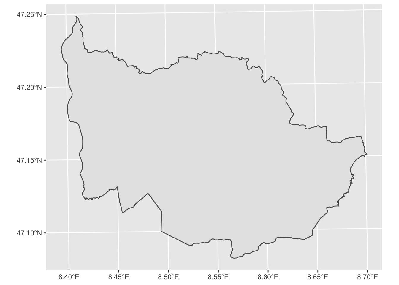
# Selecting the Canton of Zürich
zurich <- filter(kantonsgebiet, NAME == "Zürich")
ggplot(zurich) + geom_sf()  # depicting the Canton of Zurich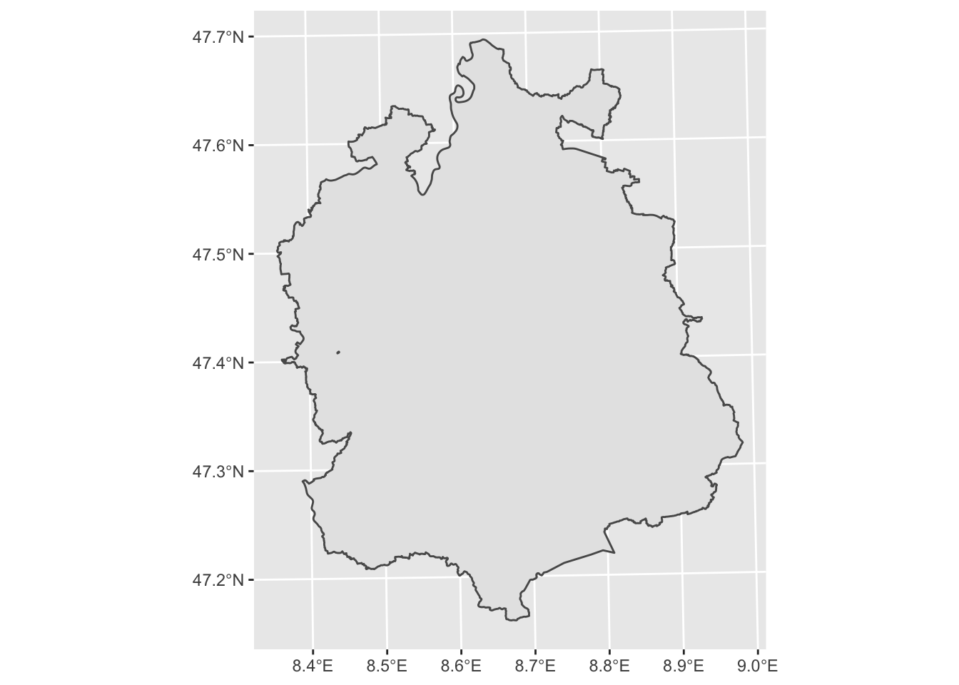
# merging the two sf objects
merged <- rbind(zug, zurich)
ggplot(merged) + geom_sf()  # depicting the product of the merge operation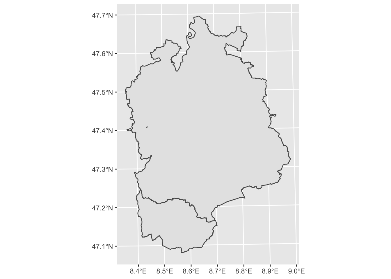
7.1.4 Dissolve
Dissolve in ArcGIS pro serves as a basic tool for aggregating features based on specified attributes. In R the respective operation could be easily performed using some basic functionalities of the sf package. In the example below we use again the dataset that depicts all the 26 Cantons of Switzerland. Our aim is to transform the given dataset to one unified spatial polygon.
# The study area from the previous example
head(kantonsgebiet)
## Simple feature collection with 6 features and 1 field
## geometry type: POLYGON
## dimension: XY
## bbox: xmin: 2494306 ymin: 1075268 xmax: 2833858 ymax: 1268609
## projected CRS: CH1903+ / LV95
## NAME geometry
## 1 Graubünden POLYGON ((2735216 1194955, ...
## 2 Bern POLYGON ((2595242 1169313, ...
## 3 Valais POLYGON ((2601808 1136117, ...
## 4 Vaud POLYGON ((2555093 1138713, ...
## 5 Ticino POLYGON ((2727359 1119219, ...
## 6 St. Gallen POLYGON ((2716175 1240719, ...ggplot(kantonsgebiet) + geom_sf() # depicting all the 26 Cantons of Switzerland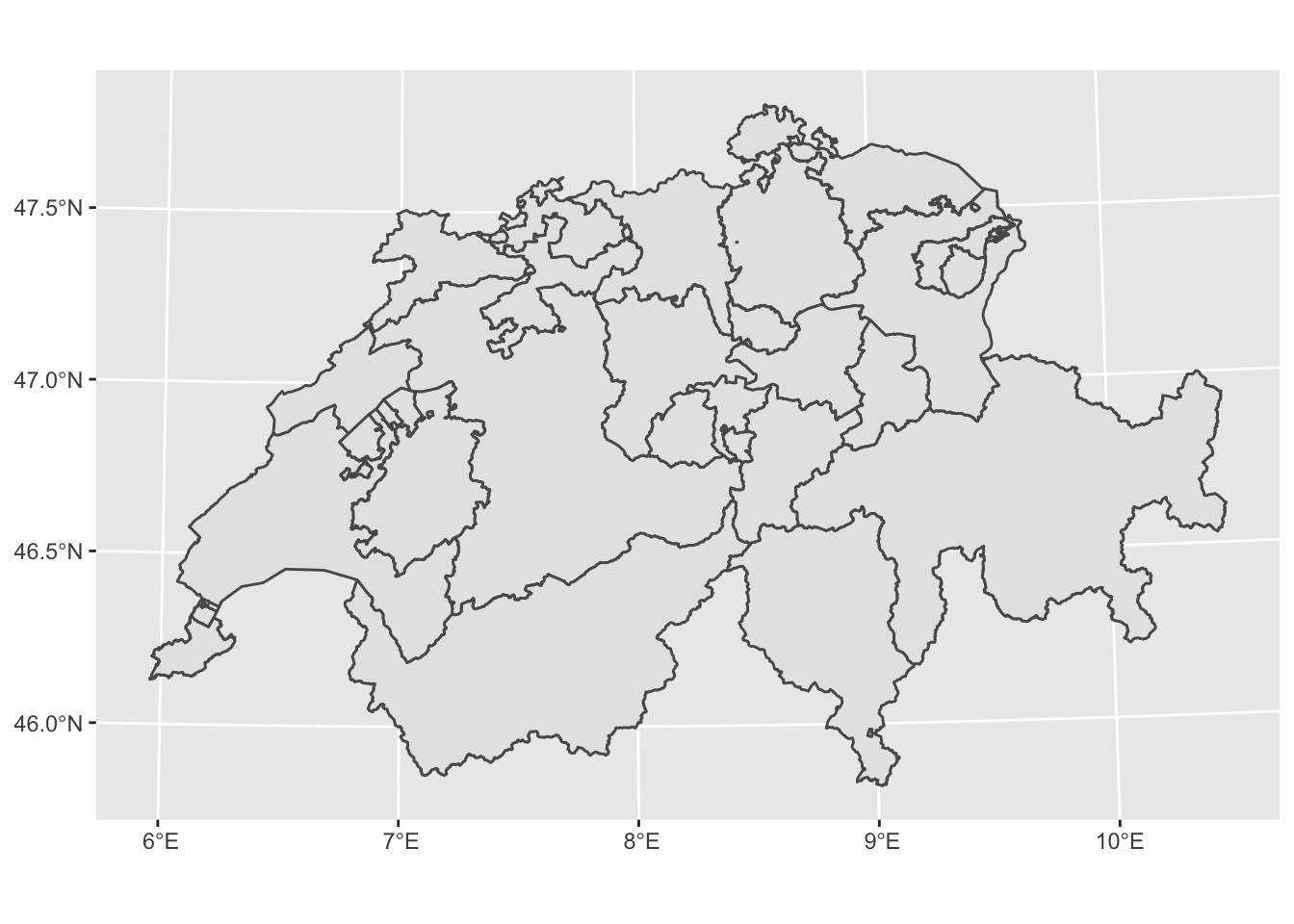
# Dissolving all the cantons into one unified area
kantonsgebiet_dissolved <- st_union(kantonsgebiet)  # use of the sf__st_union() function
head(kantonsgebiet_dissolved)
## Geometry set for 1 feature
## geometry type: POLYGON
## dimension: XY
## bbox: xmin: 2485410 ymin: 1075268 xmax: 2833858 ymax: 1295934
## projected CRS: CH1903+ / LV95# Plot the dissolved output
ggplot(kantonsgebiet_dissolved) + geom_sf()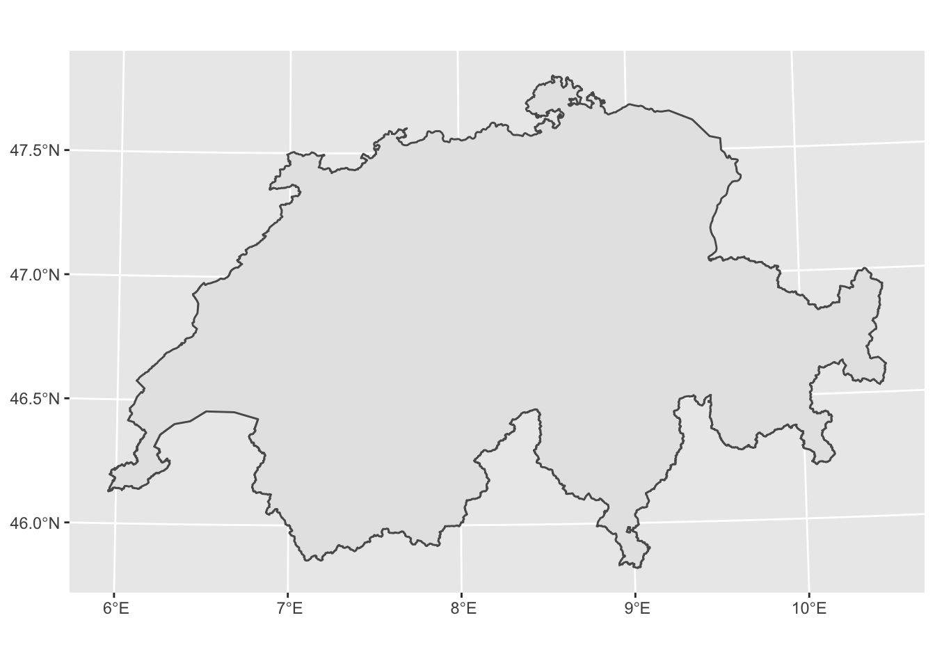
7.1.5 Find Identical
In ArcGIS pro Find Identical tool identifies records in a feature class or table that have identical values in a list of fields. As an outcome it produces a table listing those identical findings. In R we obtain a similar result for spatial features using the st_equals function of the sf package.
# create the duplicates
addDupli <- kantonsgebiet[1:3, ]

# Combine it with the original dataset (kantonsgebiet)
kantonDuplic <- rbind(kantonsgebiet, addDupli)

# Examine if there are any identical values
ident_results <- st_equals(kantonDuplic)